This document is Copyright © 2021 by the LibreOffice Documentation Team. Contributors are listed below. You may distribute it and/or modify it under the terms of either the GNU General Public License (http://www.gnu.org/licenses/gpl.html), version 3 or later, or the Creative Commons Attribution License (http://creativecommons.org/licenses/by/4.0/), version 4.0 or later.
All trademarks within this guide belong to their legitimate owners.
To this edition
Jean Hollis Weber
To previous editions
Jean Hollis Weber
Please direct any comments or suggestions about this document to the Documentation Team’s mailing list: documentation@global.libreoffice.org.
Everything you send to a mailing list, including your email address and any other personal information that is written in the message, is publicly archived and cannot be deleted.
Published May 2021. Based on LibreOffice 7.1 Community .
Other versions of LibreOffice may differ in appearance and functionality.
Some keystrokes and menu items are different on macOS from those used in Windows and Linux. The table below gives some common substitutions for the instructions in this book. For a more detailed list, see the application Help and Appendix A (Keyboard Shortcuts) to this guide.
Windows or Linux
Tools > Options menu selection
Access setup options
Control+click and/or right-click depending on computer setup
Open a context menu
Used with other keys
Exit / quit LibreOffice
Open the Sidebar’s Styles deck
Many requests for spreadsheet support are the result of using complicated formulas and solutions to solve simple day-to-day problems. For more efficient and effective solutions, use the pivot table, a tool for combining, comparing, analyzing, and summarizing large amounts of data easily. Using pivot tables, you can view different summaries of the source data, display the details of areas of interest, and create reports, whether you are a beginner, an intermediate, or an advanced user. Besides, you can create a pivot chart to view a graphical representation of the data in a pivot table.
To work with a pivot table, you need a list of raw data, similar to a database table, consisting of rows (data sets) and columns (data fields). The field names are in the first row above the list.
The data source could be an external file or database. For the simplest case, where data is contained in a Calc spreadsheet, Calc offers sorting functions that do not require the pivot table.
For processing data in lists, Calc needs to know where in the spreadsheet the list is. The list can be anywhere in the sheet, in any position. A spreadsheet can contain several unrelated lists.
Calc recognizes your lists automatically. It uses the following logic: Starting from the cell you have selected (which must be within the list), Calc checks the surrounding cells in all four directions (left, right, above, below). The border is recognized if the program discovers an empty row or column, or if it hits the left or upper border of the spreadsheet. This means that the described functions can only work correctly if there are no empty rows or columns in the list. Avoid empty lines (for example for formatting). You can format the list by using cell formats.
To make sure that Calc automatically recognizes a list correctly, check that there are no empty rows or empty columns within the list.
If you select more than one cell before creating a pivot table, then Calc’s automatic list recognition logic is not applied. Instead, Calc assumes that the pivot table is to be created using exactly the cells that you selected.
Always select only one cell before initiating creation of a pivot table. This allows Calc to automatically determine the full scope of your data list.
A relatively common source of errors is to inadvertently declare a list by mistake and then to sort that list. If you select multiple cells—for example, a whole column—then the sorting mixes up the data that should be together in one row.
In addition to these formal aspects, the logical structure of the list is also very important.
Calc lists must have the normal form ; that is, they must have a simple linear structure.
When entering the data, do not add outlines, groups, or summaries. Here are some mistakes commonly made by inexperienced spreadsheet users:
The possible data sources for the pivot table are a Calc spreadsheet or an external data source that is registered in LibreOffice.
Analyzing a list in a Calc spreadsheet is the simplest and most often used case. Lists might be updated regularly or the data might be imported from a different application.
The list data might be entered directly into the spreadsheet or copied from another file or application. You can also use a Web Page Query input filter to insert data from an HTML file, a CSV file, a Calc spreadsheet, or a Microsoft Excel spreadsheet. See Chapter 10, Linking Data, for more information.
The behavior of Calc while inserting data from a different application depends on the format of the data. If the data is in a common spreadsheet format, it is copied directly into Calc. However, if the data is in plain text format, the Text Import dialog appears after you select the file containing the data; see Chapter 1, Introduction, for more information about this dialog.
A registered data source is a connection to data held in a database outside of LibreOffice. When using a registered data source, the data to be analyzed will not be saved in the spreadsheet; Calc will always use the data from the original source. Calc can use many different data sources in addition to databases that are created and maintained with LibreOffice Base. For more information, see Chapter 10, Linking Data.
If you use pivot tables often in Calc, you might find the frequent use of the built-in menu paths inconvenient.
In some cases built-in keyboard shortcuts are already defined; see Appendix A, Keyboard Shortcuts . An example is the F12 function key, which groups a selected data range. In some other cases, the built-in toolbars already provide relevant icons. An example is the Insert or Edit Pivot Table icon on the Standard toolbar.
In addition to using the built-in keyboard shortcuts and toolbar icons, you can also define your own. See Chapter 14, Setting up and Customizing, for instructions.
If you want Calc to automatically determine the full extent of the raw data list, then select a single cell within this list. If you want to explicitly define the extent of the raw data list, then select all relevant cells.
With the cell (or cells) selected, create the pivot table by selecting Insert > Pivot Table on the Menu bar, selecting Data > Pivot Table > Insert or Edit on the Menu bar, or click the Insert or Edit Pivot Table icon on the Standard toolbar.
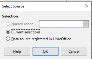
Calc displays the Select Source dialog (Figure 2), where you can choose between using the selected data cells, a range of cells that has already been named, or a data source that has already been registered with LibreOffice.
See Chapter 13, Calc as a Database, for more information about named ranges. See Chapter 10, Linking Data, for more information about linking to registered data sources.
Figure 1: Select Source dialog
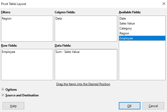
Click OK on the Select Source dialog to display the Pivot Table Layout dialog, which is described in the next section.
The function of the pivot table is managed in two places: first, in the Pivot Table Layout dialog; and second, through manipulations of the result in the spreadsheet. This section describes the Pivot Table Layout dialog in detail.
To access the Pivot Table Layout dialog again after initial creation of a pivot table, left-click in any cell of the pivot table. Then select Insert > Pivot Table on the Menu bar, or select Data > Pivot Table > Insert or Edit on the Menu bar, or click the Insert or Edit Pivot Table icon on the Standard toolbar, or right-click in any cell of the pivot table and select the Properties option in the context menu.
In the Pivot Table Layout dialog (Figure 2) are four areas that show the layout of the resulting pivot table:
Besides these four areas is another area labeled Available Fields containing the names of the fields in the source data list. To choose a layout, drag and drop the fields from the Available Fields area to the other four areas.
The Data Fields area must contain at least one field. Advanced users can use more than one field here. For the fields in the Data Fields area, an aggregate function is used. For example, if you move the Sales Value field into the Data Fields area, it initially appears there as Sum – Sales Value .
Figure 2: Pivot Table Layout dialog
Row and column fields indicate from which groups the result will be sorted. Often more than one field is used at a time to get partial sums for rows or columns. The order of the fields gives the order of the sums from overall to specific.
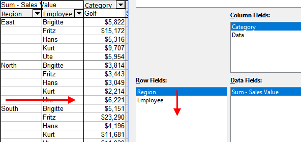
For example, if you drag Region and Employee into the Row Fields area, the sum will be divided into the regions. Within the regions will be the listing for the different employees (Figure 3).
Figure 3: Field order for analysis and resulting layout of pivot table
Fields that are placed into the Filters area appear at the top of the resulting pivot table as a drop-down list. The summary in the result takes into account only that part of the base data that you have selected. For example, if you include Employee in the Filters area, you can filter the result shown for each employee.
To move a field from an area, just drag it to a new area. To remove a field from the Filters , Column Fields , Row Fields , or Data Fields areas, drag it to the Available Fields area.
To rapidly move a selected field from one area of the Pivot Table Layout dialog to another, press the Alt+letter on the keyboard that corresponds to the underlined letter in the target area’s label.
By default, Calc inserts a Data field into the Column Fields area. The Data field can be moved between the Column Fields and Row Fields areas as required. Depending on its position within the list of fields in its area, the Data field may lead to a button labeled Data appearing in the results of the pivot table, affecting the layout of the results. If you do not wish to use this facility, simply place the Data field at the bottom of the list of fields in its area.
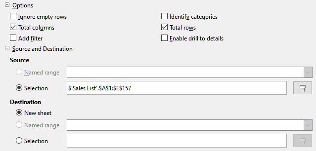
To expand the Pivot Table Layout dialog and show more options, click the expansion symbol (plus or triangle sign) adjacent to the Options and Source and Destination labels (Figure 4).
Ignore empty rows
If the source data is not in the recommended form, this option tells the pivot table to ignore empty rows.
Figure 4: Expanded area of the Pivot Table Layout dialog
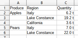
With this option selected, if the source data has missing entries in a list and does not meet the recommended data structure (as in Figure 5 for example), the pivot table adds it to the listed category above it. If this option is not chosen, then the pivot table inserts (empty) .
Figure 5: Example of data with missing entries (blank/empty values) in Column A
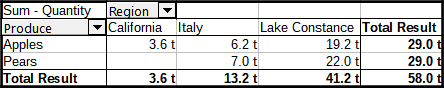
The option Identify categories ensures that in this example rows 3 and 4 are included for Apples and that row 6 is included for Pears (Figure 6).
Figure 6: Pivot table result with Identify categories selected
Without category recognition, the pivot table shows an (empty) category (Figure 7).
Figure 7: Pivot table result without Identify categories selected
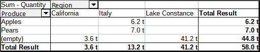
Logically, the behavior with category recognition is better. A list showing missing entries is also less usefulbecause you cannot use functions such as sorting or filtering.
Total columns, Total rows
With these options, you can decide if the pivot table shows an extra row with the sums of each column, or if it adds on the very right a column with the sums of each row. In some cases, an added total sum is meaningless, for example, if the entries are accumulated or the result of comparisons.
Use this option to add or hide the cell labeled Filter above the pivot table results. This conveniently provides additional filtering options within the pivot table. For more information, see “Filtering” below.
The filtering provided through the Add filter option is independent of the filtering provided by including fields in the Filters area of the Pivot Table Layout dialog.
Enable drill to details
With this option enabled, if you double-click on a single data cell in the pivot table result, including a cell produced from Total columns or Total rows , a new sheet opens giving a detailed listing of the individual entry. If you double-click on a cell in either a row or column field area, the Show Detail dialog opens (Figure 39). If this function is disabled, the double-click will keep its usual edit function within a spreadsheet. For more information, see “Drilling (showing details)” below.
The Selection field in this area shows the sheet name and the range of cells containing the raw data for the pivot table. If the source spreadsheet contains any named ranges, these can be selected through the Named range option.
The controls in this area define where the result will be shown.
Selecting New sheet adds a new sheet to the spreadsheet file and places the results there. The new sheet is named using the format Pivot Table_sheetname_X ; where X is the number of the table created, 1 for first, 2 for the second, and so on. For a sheet named Sales List, the new sheet for the first pivot table produced would be named Pivot Table_Sales List_1 . Each new sheet is inserted next to the source sheet.
If the target spreadsheet contains any named ranges, these can be selected with the Named range option.
The Selection field in this area shows the sheet name and the range of cells for the pivot table’s results.
To display the pivot table on the same sheet as the raw data, check the Selection option in the Destination area, click the Shrink button to the right of the Selection field, click at an appropriate cell in an empty area of the sheet, click the Expand button, and click OK on the Pivot Table Layout dialog.
The options discussed in the previous section are valid for the pivot table in general. You can also change settings for any field that is currently included in the pivot table layout. Change a field’s settings by double-clicking that field within the Filters , Column Fields , Row Fields, or Data Fields areas of the Pivot Table Layout dialog. Double-clicking a field within the Available Fields area has no effect. The options available for fields in the Data Fields area differ from those for fields in the other three areas.
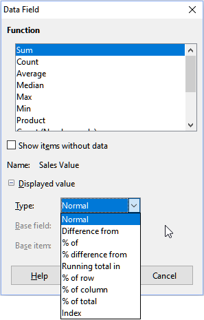
Double-click a field in the Data Fields area of the Pivot Table Layout dialog to access the Data Field dialog shown in Figure 8.
In the Data Field dialog, you can select the function to be used to accumulate the values from the data source. While you often use the Sum function, other functions (like standard deviation or a counting function) are also available. For example, the counting function can be useful for non-numerical data fields.
Select the Show items without data option to include empty columns and rows in the results table.
Click the expansion symbol (plus sign or triangle) to expand the Displayed value section of the dialog.
Figure 8: Expanded dialog for a data field
In the Displayed value section, you can choose other possibilities for analysis using the aggregate function. Depending on the setting for Type , you may have to choose definitions for the Base field and Base item .
Figure 9: Example choices for Base field and Base item
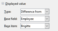
Table 1 lists the possible types of displayed value and associated base field and base item, together with notes on usage.
Table 1: Description of Displayed value options on the Data Field dialog